![]() Click to view article in PDF format.
Click to view article in PDF format.
GCInstantaneous Seismic Attributes Calculated by the Hilbert Transform*
Bob Hardage1
Search and Discovery Article #40563 (2010)
Posted July 17, 2010
*Adapted from the Geophysical Corner column, prepared by the author, in AAPG Explorer, June, 2010, and entitled “Thin Is In: Here’s a Helpful Attribute”. Editor of Geophysical Corner is Bob A. Hardage ([email protected]). Managing Editor of AAPG Explorer is Vern Stefanic; Larry Nation is Communications Director. Please see closely related article “Reflection Events and Their Polarities Defined by the Hilbert Transform”, Search and Discovery article #40564.
1Bureau of Economic Geology, The University of Texas at Austin ([email protected])
Geological interpretation of seismic data is commonly done by analyzing patterns of seismic amplitude, phase and frequency in map and section views across a prospect area. Although many seismic attributes have been utilized to emphasize geologic targets and to define critical rock and fluid properties, these three simple attributes – amplitude, phase and frequency – remain the mainstay of geological interpretation of seismic data.
Any procedure that extracts and displays any of these seismic parameters in a convenient and understandable manner is an invaluable interpretation tool. A little more than 30 years ago, M.T. Taner and Robert E. Sheriff introduced the concept of using the Hilbert transform to calculate seismic amplitude, phase and frequency instantaneously – meaning a value for each parameter is calculated at each time sample of a seismic trace. That Hilbert transform approach now forms the basis by which almost all amplitude, phase and frequency attributes are calculated by today’s seismic interpretation software
| |
|
|
The action of the Hilbert transform is to convert a seismic trace x(t) into what first appears to be a mysterious complex seismic trace z(t) as shown on Figure 1. In this context, the term “complex” is used in its mathematical sense, meaning it refers to a number that has a real part and an imaginary part. The term does not imply that the data are difficult to understand. This complex trace consists of the real seismic trace x(t) and an imaginary seismic trace y(t) that is the Hilbert transform of x(t). On Figure 1 these two traces are shown in a three-dimensional data space (x, y, t), where t is seismic time, x is the real-data plane, and y is the imaginary-data plane. The actual seismic trace is confined to the real-data plane; the Hilbert transform trace is restricted to the imaginary-data plane.
These two traces combine to form a complex trace z(t), which appears as a helix that spirals around the time axis. The projection of complex trace z(t) onto the real plane is the actual seismic trace x(t); the projection of z(t) onto the imaginary plane is the Hilbert transform trace y(t). At any coordinate on the time axis, a vector a(t) can be calculated that extends perpendicularly away from the time axis to intercept the helical complex trace z(t) as shown on Figure 2. The length of this vector is the amplitude of the complex trace at that particular instant in time – hence the term “instantaneous amplitude.” The amplitude value is calculated using the equation for a(t) shown on the figure.
The orientation angle Ф(t) that defines where vector a(t) is pointing (Figure 2) is defined as the seismic phase at time coordinate t – hence the term “instantaneous phase.” Numerically, the phase angle is calculated using the middle equation listed on Figure 2. As time progresses, vector a(t) moves down the time axis, constantly rotating about the time axis as it maintains contact with the spiraling helical trace z(t). Mathematically, frequency can be defined as the rate of change of phase. This fundamental definition allows instantaneous frequency ω(t) to be calculated from the time derivative of the phase function as shown by the bottom equation on Figure 2.
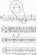
The calculation of these three interpretation attributes – amplitude, phase and frequency – are illustrated on Figures 3 and 4. Application of the three equations listed on Figure 2 yields first the instantaneous amplitude for one seismic trace x1(t) (Figure 3), and then instantaneous phase and frequency are shown on Figure 4 for a different seismic trace x2(t). Note that the instantaneous frequency function is occasionally negative – a concept that has great interpretation value, as has been discussed in a previous article (Interpretation Value of Anomalous (‘Impossible’) Frequencies, Search and Discovery article #40286). For those of you who click on a menu choice to create a seismic attribute as you interpret seismic data, you now see what goes on behind the screen to create that attribute.
Taner, M.T. and Robert E. Sheriff, 1977, Application of Amplitude, Frequency, and Other Attributes to Stratigraphic and Hydrocarbon Determination: Section 2. Application of Seismic Reflection Configuration to Stratigraphic Interpretation, AAPG Memoir 26, p. 301-327.
Copyright © AAPG. Serial rights given by author. For all other rights contact author directly. |