![]() Click to view article in PDF format.
Click to view article in PDF format.
PS![]() 3-D
3-D![]() Exploration
for Remaining Oil Using Historical Production Data
Exploration
for Remaining Oil Using Historical Production Data
Yun Ling1, Xuri Huang2, Desheng Sun1, Jun Gao1, and Jixiang Lin1
Search and Discovery Article #40399 (2009)
Posted April 10, 2009
* Adapted from oral presentation at AAPG International Conference and Exhibition, Cape Town, South Africa, October 26-29, 2008.
1BGP, CNPC, Zhuozhou, China (mailto:[email protected])
2Golden Eagle Int'l, Inc., Beijing, China
3D and 4D (or time-lapse) seismics are techniques commonly used for exploration and reservoir exploitation. Increasingly, time-lapse seismic is becoming a more popular tool for reservoir development and management. However, its application is constrained by reservoir conditions, production mechanisms and seismic data repeatability. The technique of 3D exploration for remaining oil with historical production data (3.5D) uses high quality 3D seismic data, acquired after a certain period of reservoir production, and integrates it with historical production data to provide information for reservoir dynamics, such as the identification of additional resources and the delineation of remaining oil. In integrating the 3D seismic with historical production data, the 3D seismic data are time-stamped and then related to the reservoir dynamics. This enables 3D seismic data to represent reservoir dynamics in time. The method is applied to an onshore field in Western China. The result shows that the 3.5D seismic approach can identify reservoir potentials and remaining oil.
|
Back in the late 30s, 3D wave propagation was investigated based on multiple 2D lines in different directions and wave propagation geometries (Rock, 1938). After the 50s, 3D seismic reflection and imaging were discussed based on physical 3D models. In the mid-70s, the first 3D seismic survey was acquired in the Gulf of Mexico (Dahm and Graebner, 1982). It was observed in the lab that a large velocity change can occur in rocks with heavy oil if the oil is replaced by steam (Nur et al., 1984). From the late 80s, the application of time-lapse seismic was investigated (Robert and Terrance, 1987). With hundreds of field applications in the last decade, time-lapse seismic has become an industry-wide tool for reservoir monitoring (Lumley, 2001). However, offshore and onshore applications have not been evenly balanced. Time-lapse seismic has been successfully implemented in offshore areas, especially in the North Sea and the GOM. It has also been successful in some onshore areas where there are shallow, heavy oil reservoirs, especially in Canada. Non-repeatable noise in time-lapse seismics at land fields is a key issue. 3D legacy data always reflect differences in geometries, acquisition directions, source/receiver types and their locations, surface equipment, and surface conditions. As for processing, the differences can include the processing flow, parameters, algorithms, and the software system itself (Ross et al., 1996). The non-repeatability from acquisition and processing makes it difficult for 3D time-lapse seismics to be applied to onshore fields, especially to thin interbedded reservoirs. Based on research conducted at an onshore field, we propose a 3.5D seismic method to obviate these problems.
Background of Geology and Seismic
Geology background: The field is on a monoclinal structure that forms a lithological trap for the reservoir, with depths between 3230-3480 m and sand thicknesses ranging from 3 to 5 m. The field has been in production since 1991, with water cut around 60% at present.
Seismic
acquisition and processing:
The 3D survey conducted in the
field is located in the northwest margin of the Jungar basin. The
surface is mainly covered with sand dunes of 3-20 m in height and
some farmland on the eastern side. The main parameters of the survey
geometry are as follows: Spread, 12 lines x 10 shots; Fold, 60; Bin
size, 12.5 m x 12.5 m. The processing workflow includes amplitude
preservation, source/receiver statistical deconvolution, velocity
picking, statics, and NMO+DMO+
Reservoir Structure and Depositional Study
Figure 1a is a seismic section across the reservoir, which is flattened at the bottom of the Jurassic. From this section we can see that the deposition before the Jurassic has an erosional period of exposure, with volcanic activity in the deeper formation. The Jurassic formation contacts its underlying formation as an angular unconformity. Above the unconformity, the Jurassic formation starts to subside in the southern part.
This leads to a paleotopography with a high in northwest, and a low in the southeast (see Figure 1b). Sedimentary deposition starts in the early Jurassic (J1b). This period has three sub-cycles of deposition as marked in Figure 1b by the deep to light yellowish colors for the three superimposed sedimentary units. The sediment source is from the northwest. After this period, the southeast continues to subside and leads to the formation of the mid-Jurassic deposition (J2x). J2x has two sub-cycles of deposition that form two superimposed sedimentary units, with the source in the northwest. In the late Jurassic (J3q) there are two sub-cycles of deposition (see Figure 1b marked with deep or light color) that are thicker in the southeast than in the northwest. In the seismic sections, a foreset reflection can be observed clearly in the northwest. This indicates that the sediments are from the northwest.
Figure 1c shows the present structure from the seismic data. From Figure 1c and the above structural evolution discussion, we conclude, that with a good cap rock, the reservoir mainly has onlap and unconformity lithological traps.
Based on the structural and depositional evolution study, the seismic waveform clustering attribute is generated as shown in Figure 2 . The mid-to-light blue colored region indicates a region of alluvial deposition. An uplift (the white line in Figure 2) separates it from the adjacent depositional region. These two zones form two major depositional regions. From the depositional analysis, the J3q formation mainly forms onlap traps. On the other hand, the J1b and J2x formations mainly form unconformity traps.
Historical Production Data Study
Obviously, the preceding structural and depositional discussion, which is based only on high quality 3D seismic data, cannot characterize reservoir dynamics. The key to 3.5D seismic is to further characterize the reservoir using dynamic data such as historical production data. Figure 3 is the spatial evolution of cumulative oil production. The well locations and cumulative oil production map of the early stage (1990) show that the field development starts in the south. It then expands to the north with time, and continues with the drilling of most of the production wells until 1994. At that point, most wells with high cumulative oil production are in the south (the big red circles in Figure 3 , 1994). Starting in 1996, the cumulative oil production in the north increases every year. At the same time, the production in the south starts to decline. It also shows that water production starts to increase in the south. In 2006, the cumulative production in the south is still slightly higher than that in the north, and the cumulative production in the west is higher than that in the east. Also, Figure 3 shows that the wells near the field boundaries have relatively lower oil production, which implies that they have encountered the oil/water contact. Figure 4 further shows the evolution of the cumulative water production from each well. From the maps before 1994, observe that the high water production areas are mainly located in the south and south-east of the field (the blue areas in Figure 4). This implies that the water invasion is from the south-eastern direction. The variations from 1996 to present give further evidence. In addition, a water invasion path in the north of the field can also be identified. By 2006, the field had been divided into three low water-cut oil production regions (the red areas in Figure 4) and three high water-cut regions (the blue areas in Figure 4). Comparing the evolution of the cumulative oil production (Figure 3) with the water production (Figure 4), we see that there was a higher cumulative oil production in the southeast in the early stages of field development. At present, most regions have become high water-cut areas except for the red areas shown in Figure 4 .
Interpretation of 3D with Historical Production Data
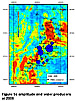
Based on the interpretation of 3D seismic data and of the dynamic data, Figure 5a shows the combined result of overlaying the dynamic data with 3D seismic amplitudes. As shown in Figure 5a , the low water producers are located in regions where the seismic amplitudes are high, and the high water producers are located in low amplitude regions in 2006. This indicates a high correlation between the water producers and seismic amplitudes. However, as shown in Figure 5b (3D seismic amplitude with cumulative oil before 2006), wells with high cumulative oil are not located at places of high 3D seismic amplitude. Wells with low cumulative oil do not always overlie regions of low seismic amplitude either. This suggests that the high-resolution 3D seismic data acquired in 2006 has been changed by fluid substitution. Thus, through this study, 3D seismic data have been characterized dynamically. To differentiate from time-lapse seismic, this can be called a 3.5D seismic approach. With the structural study of the 3D seismic data and further integration of historical production data, the aquifer invasion is mapped and the remaining potential areas are identified in Figure 6 . The water invaded from the southeast. In the north, two aquifers invaded along two paths in the J2x formation. The unexplainable Well A, as mentioned before, is located in a different sedimentary region than the field’s major producing region. The area of the remaining potential in the Well A region is estimated to be 1.5 km2. The questionable Well B is located in the same facies as that of the major production region, but it produces from a different sand body. The potential for this region has an area of 1.1 km2.
Based on a case study, a technique of 3D exploration for remaining oil using historical production data (3.5D) has been proposed and demonstrated. Compared with the workflow of time-lapse seismics, whose success depends on reservoir conditions, production mode and seismic repeatability, the workflow of our method is more practical, especially for onshore fields with thin interbedded reservoirs. The results show that reservoir dynamics can be well characterized with the seismic data acquired in producing fields, by means of effective amplitude preservation processing, structural and sedimentary studies, and integration of 3D and historical production data. This addresses the repeatability requirement for 3D time-lapse seismic and the requirement for good legacy 3D seismic data. In turn, it reduces the cost of exploring for remaining oil. The multi-disciplinary integration of seismics, geology, and reservoir engineering will greatly improve the 3.5D seismic technique and make it more effective.
Dahm, C.G. and R.J. Graebner, 1982, Field development with three-dimensional seismic methods in the Gulf of Thailand-A case history: Geophysics, V. 47/2, p. 149-176.
Lumley, D.E., 2001, Time-lapse seismic reservoir monitoring: Geophysics, V. 66/1, p. 50-53.
Nur, A, C. Tosaya, and D.V. Thanh, 1984, Seismic monitoring of thermal enhanced oil recovery processes: 54th Annual International Meeting Society Exploration Geophysists, Expanded Abstracts, Session RS.6.
Robert J.G. and J.F. Terrance, 1987, Three-dimensional seismic monitoring of an enhanced oil recovery process: Geophysics, V. 52/9, p. 1175-1187.
Rock, S.M, 1938, Three dimensional reflection control: Geophysics, V. 3/4, p. 340-348.
Ross, C.P, G.B. Cunningham, and D.P. Weber, 1996, Inside the cross-equalization black box: The Leading Edge, v. 15, p. 1233-1240.
|