Click to view abstract and references in PDF format.
For faster opening of the posters, right click on the links below to download files to your computer
![]() Poster 1 (86 mb)
Poster 1 (86 mb)
![]() Poster 2 (5 mb)
Poster 2 (5 mb)
![]() Poster 3 (97 mb)
Poster 3 (97 mb)
PSApplication of Mechanical Stratigraphy to the Development of a Fracture-Enhanced Reservoir Model, Polvo Field, Campos Basin, Brazil*
Michael Gross2, T.C. Lukas2, and Peter Schwans1
Search and Discovery Article #20080 (2009)
Posted October 15, 2009
*Adapted from poster presentation prepared for AAPG Annual Convention, Denver, Colorado, June 7-10, 2009. See companion article,
“Development Challenges in a Fracture-Enhanced Carbonate Grainstone Reservoir, Polvo Field, Brazil - from Reservoir Characterization to Dynamic Model”, Search and Discovery Article #20079 (2009).
Note: Numbers in parentheses after headings and figure captions represent numbered sections of poster presentation.
1 International Exploitation, Devon Energy, Houston, TX ([email protected]).
2 Consultant— Gross--Department of Earth Science, Florida International University, Miami, FL ([email protected]); Lukas, Houston, TX ([email protected])
A fracture model was developed for a sequence of passive-margin carbonates in Polvo Field, Campos Basin, Brazil, by applying concepts of mechanical stratigraphy to datasets derived from core, image logs and 3D seismic surveys. Upper Cretaceous carbonate rocks of the Quissama Member of the Macaé Formation include a highly porous and permeable grainstone reservoir facies underlain by various combinations of wackestone, packstone and grainstone. Systematic description of ~100m of core from a vertical well reveals a complex relationship between brittle deformation and diagenetic processes related to burial and compaction. Fractures and fabrics were subdivided into twelve distinct categories, with identification of four major mechanical units based on their vertical distribution.
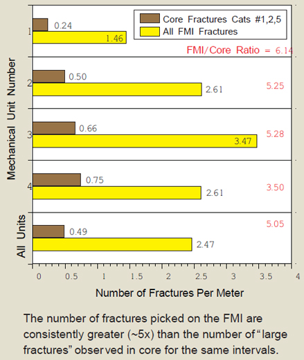
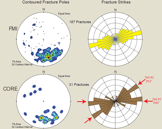
Thirty-one of 126 fractures measured in core can be precisely matched to features interpreted independently on the FMI log, allowing verification of the orientations of prominent fracture sets and establishing criteria to identify bed-confined and throughgoing fractures on image logs. The latter were used to map the occurrence of hierarchical fracture populations in FMI logs from two horizontal wells by distinguishing among bed-confined, incipient throughgoing, and mature throughgoing fractures. A conceptual model for the fractured reservoir was developed by incorporating attributes of ~ 3000 fractures identified on FMI logs, including computed apertures, into the mechanical stratigraphy established from core description, which was then correlated to seismically mapped facies. Ranges for spacing, height, length and aperture were estimated for each fracture set and mechanical unit based on scaling relations, bed thicknesses and relative strain magnitudes, providing important constraints on subsequent DFN models and reservoir flow simulations
|
|
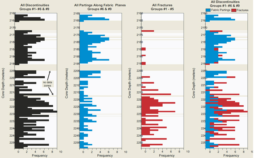
Figures 1-1, 1-2, 1-3, 1-4, 1-5, 2-1, and 2-2 The Four Main Mechanical Units (9) Units #1 -#4 A mechanical stratigraphy was developed, based on the physical properties and vertical distribution of the 11 categories of fractures and fabrics observed in core. Mechanical Unit #1 Grainstone reservoir facies characterized by thick mechanical layers, low fracture frequency, and a planar compactional fabric of mechanical origin. Mechanical Unit #2 Wackestone non-reservoir facies characterized by numerous clusters of stylolites and dissolution seams that dramatically reduce matrix permeability. Considered a leaky aquitard. Mechanical Unit #3 Packstone-to-grainstone lithology, with abundant small fractures and numerous oil-stained fracture surfaces. Many steeply inclined stylolites were reactivated as extensional fractures that accommodate fluid flow. This unit is a potential fractured reservoir, depending upon the degree of fracture connectivity. Mechanical Unit #4 Similar to overlying MU #3, except for a marked reduction in small fractures and only minor oil staining. Fracture Frequency and Mechanical Unit (Figure 2-3)
The lowest fracture frequency is in MU #1 (the grainstone reservoir), whereas the highest fracture frequency is observed in MU #3. MU#3 is characterized by an abundance of small hairline fractures. MU #2, #3 and #4 have about the same frequency of large fractures.
Fractures in Core and Features on FMI
Hydrologic Properties Inferred from Core Analysis (15)
Relative Fracture Transmissivity (Figures 2-8, 2-9, 2-10, 2-11, and 2-12; Table 2-1) A transmissivity category was assigned to each discontinuous feature observed in core, whether a fracture or fabric plane. The categories ranged from zero (impermeable) to 3 (highly transmissive) and were assigned based on the size of the feature, aperture or width, surface roughness, evidence for past fluid flow, secondary mineralization and presence of insoluble residue. Typically a major open fracture or reactivated stylolite received high values (e.g., 2.5, 3) whereas small hairline fractures received low values (1). Intact clusters of stylolites, which likely serve as impermeable flow barriers, received values of zero (0). Next a “relative fracture transmissivity” was calculated using an exponential multiplier consistent with theory of fracture flow. Flow through fractures is commonly modeled using the “cubic law” which assumes that volumetric flow rate is proportional to the cube of the fracture aperture:
Q = WΔgb3/12 Q = volumetric flow rate W = fracture length Δ = fluid density g = acceleration of gravity b = fracture aperture
Δh/ΔL = hydraulic gradient The relative transmissivity for an individual feature was calculated as the cube of the assigned transmissivity category. Thus, a fracture with an assigned transmissivity category of 2 has a relative fracture transmissivity multiplier of 8. “Fracture transmissivity” in the upper section (MU#1) is dominated by flow along partings of mechanical compaction, whereas in the lower section (MU#2-4) it is controlled by fractures. The overwhelming majority of transmissivity in the lower section is through the large fractures, despite the much greater abundance of small fractures (a function of the cubic multiplier). Compare transmissivity plots here to plots of fracture frequency in section 8 (Figure 2-2) Oil Staining on Fractures and Partings (Figures 2-13 and 2-14) An important indicator of a fractured reservoir is the occurrence and degree of oil staining on fracture surfaces. Where possible, both the occurrence (presence or absence) and degree of oil staining were noted for each planar feature observed in core. The degree of oil staining on a fracture or fabric surface was assigned a numeric value as follows: 0=no oil staining 1=minor (patch) oil staining 2=partial oil staining 3=complete oil staining The occurrence of oil staining is quantified in histograms as the number (frequency) of oil-stained fractures per meter of core depth. The degree of oil staining is quantified as the numeric staining average of all features (stained and unstained) per meter of core depth, and is presented on a color-coded scale bar. Note in MU#1 the abundant oil staining along numerous fabric partings with a high degree of staining. This may indicate potential to extend the reservoir below the surface of matrix saturation. Note the lack of oil staining in MU#2, consistent with behavior as an impermeable barrier or seal. In MU#3 there is abundant evidence for oil-stained fractures as well as oil staining along fabric partings. This suggests an active fracture-flow network with potential connectivity in the upper half of MU#3. In MU#4 oil staining on fracture surfaces is rare. Reactivated “Fractured” Stylolites (16) (Figure 2-15)
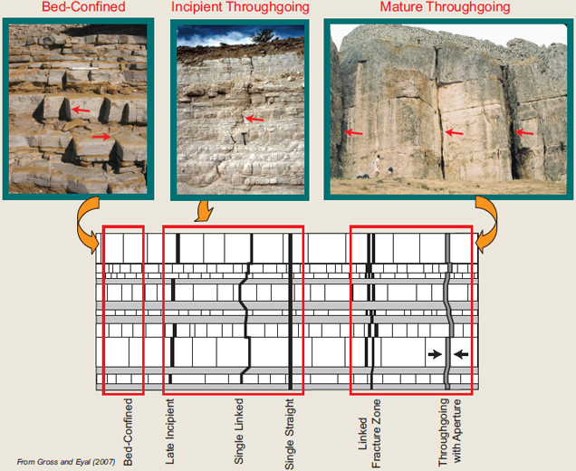
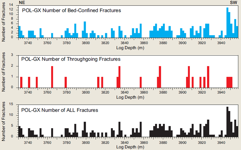
Fractures in Horizontal Wells Classification and Outcrop Analogs (17) (Figure 3-1) The POL-GX and POL-F2 horizontal wells are optimally oriented to intersect vertical fractures, which constitute the overwhelming majority of fractures encountered in the shallow-dipping strata of Polvo field. Similar to outcrop analogs, a clear scale-dependent hierarchy is observed in the fracture populations derived from image log analysis, with numerous small “bed-confined” fractures nested within the larger and more widely spaced “throughgoing fractures”. The throughgoing fractures can further be subdivided into “incipient” and “mature,” based on their degree of development. In outcrop analogs, the bed-confined fractures are contained within individual layers. Fractures terminate at bed boundaries, thus fracture heights are typically equal to bed thickness, whereas fracture lengths are unconstrained and may result in length/height ratios >> 1. Apertures of bed-confined fractures are relatively small, and their contribution to fracture flow is a function of their connectivity to the larger throughgoing fractures. Depending upon their density, bed-confined fractures may store significant quantities of hydrocarbons. Throughgoing fractures are large, multilayer structures that often represent the backbone of the fracture flow network. In many cases throughgoing fractures are zones of sub-parallel, closely spaced fracture segments. Incipient throughgoing fractures are at initial stages of linkage across bed boundaries, whereas mature throughgoing fractures are well defined zones characterized by large fracture apertures. Throughgoing fractures provide important vertical connectivity among beds that would otherwise be hydraulically isolated. By virtue of their high transmissivities and fracture connectivity, throughgoing fractures are prime targets for intersection by horizontal wellbores. Identification on Image Logs (18) (Figures 3-2 and 3-3) The three main types of fractures observed in outcrop analogs can be identified on image logs from horizontal wells. (1) Bed-confined fractures appear as discontinuous features with narrow widths, and thus are considerably less prominent than throughgoing fractures. Their terminations at stratigraphic boundaries are often observed on the image log. In many cases, numerous bed-confined fractures cluster around mature throughgoing fractures. (2) Incipient throughgoing fractures are continuous across the image log but not as prominent as the mature throughgoing fractures, and often lack a consistent width. However, their widths and continuity are much greater than for the smaller bed-confined fractures, and they do not terminate at bed boundaries. (3) Mature throughgoing fractures are distinguished by a continuous, thick band of low resistivity, indicating a consistently wide aperture relative to incipient throughgoing fractures and bed-confined fractures. Orientations of Fracture Strike (19) (Figure 3-4) Spatial Distribution of Fractures in Horizontal POL-GX Well (20) (Figures 3-5 and 3-6) There appears to be an increase in the frequency of bed-confined fractures with depth. In general, the interval can be divided into two domains: a domain of lower fracture frequency in the first (NE) section, and a domain of higher fracture frequency in the second (SW) section. The highest frequency of bed-confined fractures is associated with a fault at ~3950m (Figure 3-6). Estimates of Fracture Aperture and Aperture Distribution with Depth in Horizontal POL-GX Well (21) (Figure 3-7)
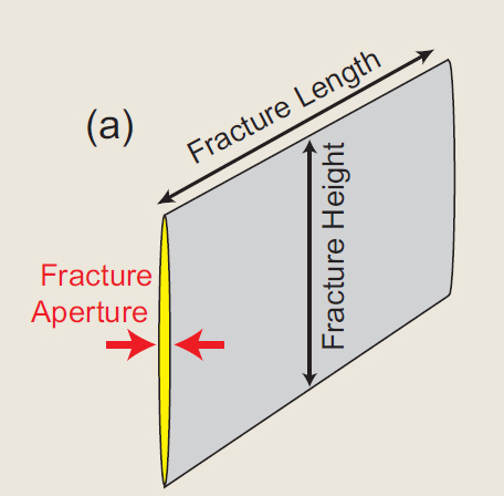
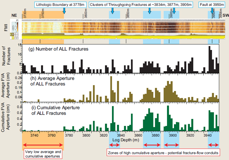
Fracture aperture refers to the width of the opening between opposing walls of a fracture, as measured perpendicular to the fracture surface. For joints, the opening is filled with gases and/or fluids, whereas for veins the volume is filled with solid mineral crystals. It is important to distinguish between “mechanical” and “hydraulic” aperture. The mechanical aperture is a geometric property of the fracture; i.e., the physical measurement of the gap between two planar surfaces (see Figures 3-7(a), 3-7(b), and 3-7(c)). The hydraulic aperture is an idealized value that is either derived empirically from the cubic law (see section 15, Panel II [Poster 2]), or alternatively assigned to represent the transmissivity of the fracture for the purpose of fluid flow modeling. Fracture apertures are not measured directly by the FMI, and hence do not represent physical measurements of the opening between fracture walls (i.e., mechanical fracture aperture). Rather, values for fracture aperture (e.g., FVA from FMI logs) are derived through an empirical equation based on the excess conductivity associated with a discrete fracture identified on the FMI (Luthi and Souhaite, 1990). Although FVA apertures derived from FMI should be used with caution when applying equations of fracture mechanics and fluid flow, the relative magnitudes of FVA fracture apertures derived from FMI logs may provide valuable insight when fracture aperture populations are compared as a function of lithology, scale, orientation, and structural position. Mean and median apertures of throughgoing fractures are nearly twice as large as for bed-confined fractures (Figure 3-7(d) and Figure 3-7(e)), a relationship that can also be seen in the scatter plot (Figure 3-7(f)). Note the clustering of bed-confined fractures adjacent to throughgoing fractures (Figure 3-7(f)). Frequency plots of number of fractures (Figure 3-7(g)), average fracture aperture (Figure 3-7(h)), and cumulative fracture aperture (Figure 3-7(i)) for 2m intervals reveal a strong dependence of aperture size on lithology and identify several potential fracture-flow zones. Models and Cross Section (Figures 3-8, 3-9, and 3-10) Gross, M.R., and Y. Eyal, 2007, Throughgoing fractures in layered carbonate rocks; GSA Bulletin, v. 119, p. 1387-1404. Luthi, S.M., and P. Souhaite, 1990. Fracture apertures from electrical borehole scans: Geophysics, v. 55, p. 821-833.
Copyright © AAPG. Serial rights given by author. For all other rights contact author directly. |