Abstract/Excerpt

Constraining Thermal Histories from Limited Data in Poorly Studied Basins

Kerry Gallagher
Géosciences, Université de Rennes 1, Rennes, France

In frontier basins, the data available is often relatively limited, and the general understanding of the thermal evolution is poor. For example, it may be that 1 or 2 wells have been drilled, and some thermal indicator calibration data are available (e.g. vitrinite reflectance, apatite fission track analyses). However, the general stratigraphy (e.g. lithologies, ages, unconformities) is perhaps not well known, and we do not have enough regional information to develop appropriate geodynamic forward model simulations for thermal maturity. In this case, we want to make the most of the available thermal calibration data, and also quantify the uncertainties associated the inferred thermal histories.

This can be achieved by using inverse methods to find the range of thermal histories consistent with the calibration data from a borehole or surface samples. In principle we can infer the thermal histories directly from the data, without needing to use subsidence/heat flow histories, which may be required when stratigraphic and lithological information are limited. Recently developed methods based around Monte Carlo simulation allow the data to determine also the complexity of the inverse models, typically defined in terms of the number of parameters required in the model to fit the data adequately. These methods have the advantage of avoiding both overinterpretation of the data and the introduction of features not really required by the data. The implementation of such methods to the thermal history problem has been described in detail by Gallagher (2012, J. Geophys. Res., doi:10.1029/2011JB008825).

Given the poor state of knowledge and the fact that the calibration data and model inputs will have uncertainty, we should allow for this when setting up an inverse model. Therefore, the approach is developed in a probabilistic (Bayesian) framework. This allows us to sample from a prior range of values and then refine this range, as we use the information available from the calibration data. Thus, a thermal history model may be initially defined in terms of the range of temperature and time values deemed acceptable. For example, we may specifiy a range of 150±150 million years, and 80±80°C. A thermal history is constructed by sampling a number of time-temperature points, drawn from the prior range, and using linear interpolation between these discrete points. The number of time-temperature points is treated as an unknown.

If we are dealing with multiple samples at different depths, we similarly specify a range on the temperature gradient (e.g. 25±15°C/km), a parameter which can change also with time. We can also build in additional specific constraints if required. For example, we may have information that loosely defines the stratigraphic age as Upper or Lower Cretaceous for example and we may have some often imprecise downhole temperature measurements as constraints on the present day thermal state in a well. Finally, the calibration data themselves are not perfect, nor are the models used to predict them. This additional source of uncertainty can be allowed for by resampling the data themselves or the predictive model parameters themselves.

As an example of the application of this methodology, we have used a well from an unidentified frontier basin. This example may be relatively typical in that many important parameters are not very well known. These include the stratigraphic ages of the sediments (which were mainly terrestrial and not fossiliferous), the age and duration of an unknown number of unconformities in the well. The available calibration data were downhole temperature measurements (with a precision of about 10%) and a suite of apatite fission track data from 14 downhole samples. A complication with the fission track is that some of the samples are clearly not totally reset after deposition, i.e. they retain an unknown component of the predepositional thermal history, which needs to be allowed for. Finally, in this case, there were no data concerning the composition of apatite, which influences the rate of annealing, and so the inferred thermal histories. In this case, we need to assume a reasonable range for the compositional parameter, and treat this as an unknown to be inferred from the data, in the same way we deal with the thermal history parameters.

The process of inferring the thermal history relies on an iterative approach, sampling model parameters (e.g. time-temperature points, temperature gradients, stratigraphic ages, apatite composition, etc.) from the specified prior ranges, or distributions. The first set of parameter values are drawn randomly from these distributions. This is known as the current model. Then the data fit (known as the likelihood) is calculated for the current modell. Subsequently, we perturb the current model by adding a random change to one or more of the parameters. This new model is known as the proposed model. We calculate the data fi for this proposed mode. Then we compare the likelihoods of the proposed and current models. If the proposed model fits the data better than the current model, the proposed model becomes the current model for the next iteration, i.e. we accept the proposed model. If not, we use simple probabilistic rules to decide whether to replace the current model with the proposed model (accept it), or not (reject it). In practice the closer the proposed model is to the current model in terms of fitting the data, the more likely it is to replace the current model (even though it does not fit the data as well). The effect of this process is to allow the iterative sampling to move around the range of acceptable model parameter values, sometimes sampling not so good models at the expense of better ones.

Qualitatively this process can be explained by considering a Gaussian distribution, which we assume to represent the true underlying distribution on a model parameter, although we do not know in advance what this distribution really looks like. To reconstruct this distribution, we can see that we want to sample values more often under the peak of the distribution (the better data fitting models). However, we also want to sample the low probability tails of the distribution every now and again, as the model parameter values have a non-zero probability. After running the sampler for many iterations, we represent the underlying distribution by plotting a histogram of all the current models sampled.

In figure 1, we show the results of the inversion for the well described earlier. Here the prior range on the time and temperature values was specified as 350±350 Ma and 70±70°C, and the temperature gradient as 30±30°C/km. We show two thermal histories, the maximum likelihood model (figure 1a) and the expected model (figure 1b). The maximu likelihood model is the one that best fits the data (in terms of the numerical value of the data fit), but may have unjustified complexity (i.e. can be overfitting the data). The expected model is effectively the weighted mean of all the thermal histories accepted during the sampling. This model will often lead to a poorer data fit than the maximum likelihood model, but is often to be preferred as it better accords to the desire that we are interested in a distribution of acceptable models, not just one “best” fit model. As we deal with distributions, we can also easily calculate the uncertainty (in terms of a 95% probability range about the expected model), as shown in figure 1b. We can see that the calibration data from the well are well explained by both models (figures 1c and 1d), and the inferred range on the compositional parameter is smaller than the input range (figure 1e).

In this presentation, I will give an overview of this new thermal history inversion methodology, demonstrating how it is implemented through a user friendly software package (QTQt), which runs on Macintosh, PC and Linux.

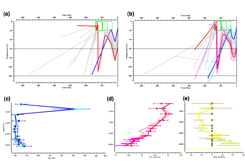
Figure 1.
(a) The inferred maximum likelihood thermal history for a suite of borehole data. The 3 time-temperature boxes at 0-20°C are the input constraints on the stratigraphic age (and deposition temperature). The oldest point in each thermal history reflects a pre-depositional component to the thermal history (required as a consequence of the samples not being totally annealed post-deposition). (b) as (a) but showing the expected thermal history, with the 95% probability range shown as the pair of thinner lines about the upper and lower thermal histories.
(c) Observed and predicted AFT (filled circles). The predicted values for the maximum likelihood and expected models are shown as thick and thin lines. Error bars (2σ are shown on the observed values and the lighter horizontal bars indicate the ±1σ range on the predicted ages for all accepted models.< /br> (d) As (c) but for the observed and predicted mean track length (MTL) values. The predicted values for the maximum likelihood and expected models are shown as thick and thin lines . Error bars are shown on the observed values and the lighter horizontal bars indicate the ±1σ range on the predicted ages< /br> (e) As (c) but for the input (squares) and predicted kinetic parameter (Dpar) values. Here there were no observed/measured values so the input value was fixed at 2±0.2μm for all samples. The error bar at the bottom of the figure shows the input range used for sampling this parameter. Note how the inferred range for each compositional parameter is less wide than the input range, implyin that there is information in the data concerning these values.< /br>

AAPG Search and Discovery Article #120098©2013 AAPG Hedberg Conference Petroleum Systems: Modeling the Past, Planning the Future, Nice, France, October 1-5, 2012