AAPG GEO 2010 Middle East
Geoscience Conference & Exhibition
Innovative Geoscience Solutions – Meeting Hydrocarbon Demand in Changing Times
March 7-10, 2010 – Manama, Bahrain

On Utilizing Functional Networks Computational Intelligence in Forecasting Rock Mechanical Parameters for Hydrocarbon Reservoirs: Methodology and Comparative Studies

Emad A. El-Sebakhy¹; Ognian Asparouhov¹; Abdulazeez Abdulraheem²; Abdul-Aziz Al-Majed²; Donghui Wu¹; Kris Latinski¹; Wade Spries¹

(1) Medical Artificial Intelligence (MEDai), Inc. an Elsevier Company, Orlando, FL.

(2) Center of Petroleum and Minerals, King Fahd University of Petroleum & Minerals, Dhahran, Saudi Arabia.

Abstract
Rock mechanical parameters of reservoir rocks play an extremely important role in solving problems related to almost all operations in oil or gas production. A continuous profile of these parameters along with the depth is essential to analyze these problems which include wellbore stability, sand production, fracturing, reservoir compaction, and surface subsidence. The mechanical parameters can be divided into three main groups: viz., elastic parameters, strength parameters, and in-situ stresses. Even the profile of in-situ stresses with depth is estimated using logs with elastic parameters as an essential input. The focus of this research is on the prediction of elastic parameters along with the depth of a given reservoir based on functional networks as a novel computational intelligence and data mining modeling scheme.
A comparative study with the most common statistical, neural networks, state equations in the petroleum engineering communities is carried out with real-industry databases. The results show that this new approach is reliable, flexible, stable, and achieves a high-quality performance.

Introduction
Rock is the “home” of oil and gas. The mechanical behavior of rock and the external factors such as insitu stresses, pore pressure, and temperature governs all aspects of completion, stimulation, and production. Identifying and estimating rock mechanical parameters for hydrocarbon reservoirs will lead to reliable achievements which lead to reliable solutions for challenge oil and gas problems.The reliable compressibility values are essential for reserves estimation, production forecasting and history matching, reservoir compaction, and permeability change and surface subsidence predictions.
Rock mechanical behavior of hydrocarbon bearing formations is very important in the oil industry.  Rock elastic properties such as Poisson ratio, Young's modulus and bulk modulus play an important role in various stages of upstream operations, such as drilling, hydraulic fracturing, and production.  Accurate knowledge of rock mechanical properties gives petroleum engineers the tool for the most efficient management of drilling, completion and production in oil or gas wells.  In addition, they are the most important pieces of information in design and management of sand production, stimulation, and wellbore instability.  Usually, those properties are measured in the laboratory through set of uniaxial and triaxial tests on cores.  However, core samples are either unavailable or expensive.  Many attempts were made to correlate those properties to well logs using either regression analysis or mathematical models, but with limited success.    This could be attributed to the fact that the rock mechanical properties are affected by numerous factors related to geological and engineering environment, and it is difficult to express these factors into a mathematical model.
A continuous profile of the properties along the depth of the reservoir is therefore generated by calibrating the dynamic elastic properties calculated from the well-log data with the static elastic properties obtained in the laboratory for selected depth points [1, 2, 3, and 4].
The calibration process plays an extremely important role in generating a reliable profile of the parameters. Currently, the conventional human expert’s reasoning process are getting replaced by both predictive data mining (DM) and artificial intelligence (AI) systems that can attack the same issues within less computational time, efficient and reliable performance. These tools are more efficient for modeling the kind of uncertainty associated with vagueness, imprecision, and/or a lack of information related to a particular problem.
Artificial neural networks, Fuzzy logic inference systems, and statistical regression have been proposed for solving many problems in the oil and gas industry, including permeability and porosity prediction, reservoir characteristics, identification of lithofacies types, seismic pattern recognition, estimating pressure drop in pipes and wells, and optimization of well production [1, 2, 3]. However, the technique suffers from numerous drawbacks, namely, the limited ability to explicitly identify possible causal relationships and the time-consumer in learning and implementation processes, overfitting, complexity, and local optima.  
Recently, functional networks have been introduced by [5, 6, 7, and 8] as a generalization of the standard neural networks. It dealt with general functional models instead of sigmoid-like ones. In Functional Networks, the functions associated with the neurons are not fixed but are learnt from the available data. There is no need, hence, to include weights associated with links, since the neuron functions subsume the effect of weights. Functional networks allow neurons to be multi-argument, multivariate, and different learnable functions, instead of fixed functions. Functional networks allow converging neuron outputs, forcing them to be coincident. This leads to functional equations or systems of functional equations, which require some compatibility conditions on the neuron functions. Functional networks have the possibility of dealing with functional constraints that are determined by the functional properties of the network model.
The main objective of this study is to investigate the capabilities of functional networks as a new artificial intelligence predictive modeling in predicting the rock mechanical properties using open hole databases. Therefore, we will be able to get over some of the standard neural neural networks limitations discussed above.
To demonstrate the usefulness of functional networks as a novel computational intelligence scheme for predicting rock mechanical parameters for hydrocarbon reservoirs, we utilized two different databases from Middle East.  The first database contains 51 well log data samples with five input variables (predictors) and the targets are: Young’s Modulus (E), Poisson’s Ration (v), Cohesion (C), Angle of internal friction (F) and Unconfined Compression Strength (UCS). The second database has 77 samples of well logs with only two input variables (DT and RHOB), with target outcomes: Young’s Modulus (E), Poisson’s Ratio (v), needed to be determined.

Literature Review
Almost all the operations of petroleum extraction involve mechanical interaction with the rock. In drilling, the knowledge of mechanical properties as well as the in-situ stress is essential for the determination of the optimum drilling path, especially in case of deviated and horizontal wells.  Knowing these properties will also help prevent wellbore collapse and optimize drilling parameters, such as mud weight for vertical as well as deviated wells. In well completion, these properties serve as an important input to optimize the perforation shot density and phasing.  In stimulation, efficient design of hydraulic fractures depends to a significant extent on the input of these parameters. The maximum sand free hydrocarbon production rate from unconsolidated sandstone reservoirs can be determined provided the material properties and the stress distribution around the wellbore is known. In Improved oil recovery, the impact of rock mechanical parameters on drilling and waterflooding is well recognized.
In view of the enormous impact of the petroleum related rock mechanics on different aspect of hydrocarbon production, the availability of a database is extremely useful and essential to any future operation related to drilling, production, and stimulation for optimization of the operation costs as well as the hydrocarbon production.
The only tool that responds to the elastic properties of the formation is the sonic logging. The sonic tool measures the characteristic propagation speed of the P- and S-waves. In an isotropic medium, only the two elastic constants, the shear modulus G and Poisson’s ratio ν are independent. They are related to the velocity of propagation of a P-wave Vp, and that of the S-wave Vs, by:

G =  rb * Vs2  ;   n = (2 Vs2 – Vp2)/ (2 Vs2 - 2Vp2)    (1)

Young’s modulus E is related to the two constants by
E = 2 G (1+ n)                                                                 (2)
There is often considerable disagreement between the static moduli obtained from conventional ‘static’ tests and the dynamic v moduli obtained from wave velocities and density of the rock. Dynamic moduli are invariably higher than static moduli [9]. The ratio of dynamic to static moduli ranges from approximately 1.5 to 3.0. Several mechanisms are responsible for these discrepancies, such as, (i) The strain magnitude effect [10, 11] and (ii) The frequency effect [12]. The more competent the rock, the less the discrepancy is. The industry has relied on the simple regression technique to calibrate sonic log derived mechanical properties with static measurements. In such methods, as discussed by [13, 14] a transfer function is obtained between the static and dynamic mechanical properties with cross plotting and curve fitting procedures.
The authors in [15] proposed the FORMEL (FORmation MEchanical Logging) model for strength profiling of weak rocks. Other approaches along similar lines have been reported in the literature. Very few studies have been conducted to predict rock mechanical properties using artificial intelligence techniques. This is partly because of the fact that artificial intelligence based approach requires a significant amount of data for training the system. The authors in [16] presented a neural network based approach to estimate the rock mechanical properties especially for wells with limited log suites. The authors in [17] employed fuzzy logic to group well log data into important datasets and discover expected and unexpected structural relationships between datasets. Using this approach he predicted rock properties along the depth of the reservoir. This research explores the possibility of utilizing functional networks to predict rock mechanical properties and their variation with the depth of a given reservoir; see [1] for more details.

Statistical Regression
Multiple linear regression attempts to model the relationship between two or more explanatory variables and a response variable by fitting a linear equation to observed data. Every value of the independent variable x is associated with a value of the dependent variable, y. The regression line for p predictors x1, x2, x3, …, xp is defined to be:

my = b0 + b1 x1 +b2 x2  + … + bp xp ,                            (3)
This line describes how the mean response my changes with the explanatory variables. The observed values for y vary about their means my and are assumed to have the same standard deviation, s. Formally, the model for multiple linear regression given n observations is:

yi = = b0 + b1 x1 +b2 x2  + … + bp xp + ei  , (4)

for i = 1….n, where ei is notation for model deviation. One approach to simplifying multiple regression equations is the stepwise procedures. These include forward selection, backwards elimination, and stepwise regression, which they add or remove variables one-at-a-time until some stopping rule is satisfied.

Artificial Neural Networks
The topology of the neural network is a graphical structure in which the nodes are the predictors and directed edges with weights are connections between neuron inputs and neuron outputs. Neural networks are characterized by the network architecture, that is, the number of layers, the number of nodes in each layer, and how the nodes are connected. The most popular kind of neural network in the industry applications is the Multilayer perceptron (MLP) network, where all nodes and layers are arranged in a feedforward manner. The first layer is called the input layer where external information is received. The last layer is called the output layer where the network produces the model solution. In between, there are one or more hidden layers which are critical for neural networks performance. All nodes in adjacent layers are connected by acyclic arcs from a lower layer to a higher layer. See [18, 19] and the references therein for more details.

Neuro-fuzzy inference systems
Fuzzy logic is an excellent tool for modeling the kind of uncertainty associated with vagueness, with imprecision, and/or with a lack of information regarding a particular element of the problem at hand. It performs well on uncertain information, very similar to the way human reasoning does. Brief details and the most common basic concepts, such as, concepts of fuzzy set theory, including fuzzy relations, fuzzification and defuzzification, construction of membership functions, and fuzzy arithmetic can be shown in [20, 21]. The Fuzzy sets are defined through their membership functions, μ, which map the elements of the considered universe to the unit interval [0,1]. The membership of an element x in the crisp set A is represented by the characteristic function mA of A, that is,
μ_A = 1, if x ∈ A;   and  μ_A = 0, if x ∈ A.  See [20, 21] and the references therein for more details.

Functional Networks Predictive Models
Functional network is a generalization of the standard neural network; it deals with generalized functional models instead of sigmoidal standard types. The initial architecture of functional network is a problem driven, i.e., it is designed based on a problem in hand. Functional networks final topology is chosen according to knowledge expertise, data domain, and information about the other properties of the neuron function such as associativity, commutativity, and invariance.  There is no need, hence, to include weights associated with links, since the neuron functions subsume the effect of weights. In addition, functional networks allow neurons to be multi-argument, multivariate, and different learnable functions, instead of fixed functions. Furthermore, functional networks allow converging neuron outputs, forcing them to be coincident. This leads to system of functional equations, which require some compatibility conditions on the neuron functions [5, 6, 7, and 8].
Functional networks modeling scheme has been utilized in solving numerous of prediction and classification problems such as regression, interpolation, and pattern recognition in medicine, flood forecasting, bioinformatics, engineering, software engineering, and business applications.
The goal of predictive data mining is to develop intelligence dynamical models for either continuous or categories outcomes to determine the relationship among set of input and output variables of a given dataset, [X1,…,Xp; Y], where X is n-by-p matrix of input variables and Y is n-by-1 vector of output variable. Let us consider the nonlinear model,

g(Y) = f(X₁,X₂,…,X_p).                                                       (5)

Assuming that g is an invertible (one-to-one and onto) function, then this nonlinear model can be written as:

Y = g^-1[f(X₁,X₂,…,X_p)]=h(X₁,X₂,…,X_p).                        (6)

Therefore, we are interested in (i) Discovering the structure of both functions: f and g in the first part or (ii) Modeling Y as a nonlinear function of  [X₁,X₂,…,X_p] in the second part.
The objective in the case of developing a predictive model for a continuous outcome is to model Y using a nonlinear function of numerous predictor variables, which is equivalent to approximate the functions f(X₁,,X₂,…,X_p) or h(X₁,,X₂,…,X_p) by linear combinations of elementary functions, that is,

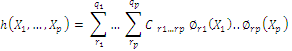
where are the parameters in the model; are families of linearly independent functions, and q_sis the number of elements in for

Development of a typical model based on functional networks involves several steps described below:

• Define the problem by specifying the initial topology based on the domain of the problem in hand;
• Simplify the chosen initial architecture using functional equations and the equivalence concept.  Check the uniqueness condition of the desired architecture.
• Gather the required data and handle multicollinearity problem along with the required quality control checks.
• Develop the learning procedures and training algorithm based either on structure or on parametric learning by considering the combinations of linear independent functions,
• , s=1,…,p to approximate the neuron functions, for  all t; where the coefficients  are the parameters of functional networks needed to be estimated. The most popular linearly independent functions in literature are:
• , or
•  or
• ,
• where m is the number of elements in the combination of sets of linearly independent function. The unknown parameters, can be learned using one of the known optimization (loss criterion) techniques, such as least squares, conjugate gradient, iterative least squares, minimax, or maximum likelihood estimation. 
• Select the best model and validate it. The selection is based on the minimum description length and some other quality measurements, such as correlation coefficients and root-mean-squared errors.  One can use the well known selection schemes, such as, exhaustive selection, forward selection, backward elimination, backward forward selection, and forward backward elimination. Once the performance of a functional networks model is satisfactory, the model is ready for use in predicting unseen datasets from real-world applications.

A typical functional network architecture is shown in Figure 1.

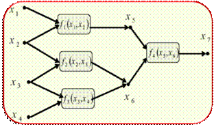
Figure 1. Typical functional network architecture.

Data Acquisition

Due to the unavailability of enough data, few studies could be undertaken to predict rock mechanical properties from wirline log data using Artificial Intelligence techniques. The latest study in this field was done by one of the authors in [1], where continuous rock mechanical properties have been predicted from log data using distinct artificial intelligence approaches, namely, neural networks and fuzzy logic inference system. The data used were 77 core samples from the same reservoir with log data. The input data were compression wave travel time (DT) and bulk density (RHOB) from wireline logs whereas the target data were Young’s Modulus and Poission ratio from core tests. The study concluded that artificial intelligence can be successfully used to predict rock mechanical properties from certain log data. It has also been concluded that the fuzzy logic has performed better than the other predictive modeling schemes. In this research, the same strategies are utilized, however more input and target data were utilized using Functional networks.

The first acquired field database with 51 samples is organized as follows:

• Core Data (Target): Complete Special Core Analysis for 51 core plugs from seven well logs across the same sandstone reservoirs: core porosity, Young’s Modulus (E), Poisson’s Ration (v), Cohesion (C), Angle of internal friction (Φ) and Unconfined Compression Strength (UCS).
• Wireline Log data (Input): Wireline openhole logs from the same wells across the same cored intervals: porosity (PHIE), bulk density (RHOB), Gamma Ray (GR), Shear Wave Velocity (DTXX), and Compression Wave Velocity (DTCO).

The second acquired field database with 77 samples is organized as follows:

• Core Data (Target): Young’s Modulus (E) and Poisson’s Ration (v).
• Wireline Log data (Input): Wireline openhole logs from the same wells across the same cored intervals:  bulk density (RHOB) and Shear Wave Velocity (DT).

The available well-log data were taken at 0.5 feet intervals which did not match the depth of the core plugs. The first step taken was to interpolate the log data to match the exact depth of the core plugs where the rock mechanical properties data were obtained. After this step was completed, all the data were merged together in one set and the depth column was removed. Therefore, the relationship between the input data (log data) and each one of the target data was found through determining the correlation coefficient of each of the parameters. The results of correlation coefficient are summarized in Table 1.

Table 1: Data with 51 samples: Correlations among core data variables and well log predictors. 

We follow the same strategy as in [1], where the authors use the wire line log parameters obtained for a selected well and the corresponding mechanical properties were determined in the laboratory on 77 core plugs at selected depth points of the same well. The input dataset for the model consisted of compression wave travel time (DT) and bulk density (RHOB) obtained from wire line logs and the target dataset consisted of Youngs Modulus (E) and Poissons Ratio (PR or ν) obtained in the laboratory.
Statistical Information about the modeling variables and their correlation coefficients are shown from Tables 2 and 3, respectively. In addition, the Cumulative Frequency Distributions (CFD) of Young’s Modulus, Poisson’s Ratio, DT, and RHOB are shown in Figure 2. Furthermore, Figures 3 and 4 show the Scatter plots of both outcomes (E and PR) versus the input parameters in both datasets, respectively, see [1] for more details.

Table 2: Data with 77 samples: Statistical quality measures.

Table 3:  Data with 77 samples - Correlation coefficients of  Young’s Modulus and Poisson’s Ratio.

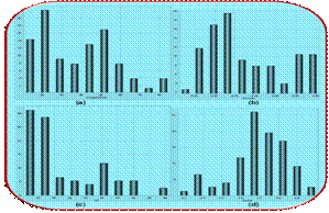
Figure 2: Data with 77 samples: Cumulative Frequency Distribution of (a) Young’s Modulus; (b) Poisson’s Ratio; (c) DT; and (d) RHOB as in [1].

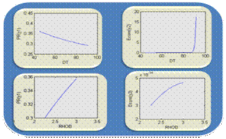
Figure 3: Data with 77 samples: Scatter plots of both outcomes (E and PR) versus the input parameters: DT and RHOB as in [1].

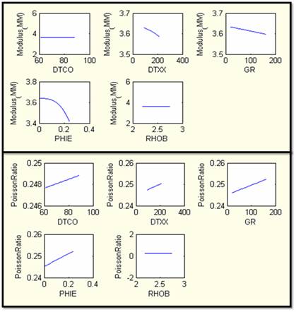
Figure 4: Data with 51 samples: Scatter plots of both outcomes (E and PR) versus predictors: DTCO, DTXX, GR, PHIE, and RHOB.

Implementation Process and Working Strategies
The available dataset is divided into two sets, viz., the training and the testing set.  The training set is used to build the model while the testing set is used to evaluate the predictive capability of that model. This division is usually done by selecting the data points in a specific order order through the use of stratifying sampling approaches.  Some of these approaches include: (i) leave-one-out, (ii) k-fold cross validation for k=10, 20…etc, and (iii) random division (70% for training and 30% for testing; or any other percentages). In the case of randomly selection, we may repeat the prediction and validations processes numerous times and then compute the quality measures discussed in the next section for the predictive models.
The input variables are normalized to make sure that they are independent of measurement units. Thus, the predictors are normalized to interval of [0,1] using the formula:

This led to a set of input variables that are independent of their measurement units. The normalized inputs are then used for all the models.

Statistical Quality Measures
To compare the performance and accuracy of functional networks forecasting learning approaches with those of other models, we made use of the most common statistical quality measures: correlation coefficient or R², root mean squared error (RMSE), Mean absolute percentage error (MAPE). The corresponding mathematical formulae for these quality measures can be briefly written follows:            

• Root Mean Squares Error: Measures the data dispersion around zero deviation:

where  is a relative deviation of an estimated value from experimental input data points, that is,

• Correlation Coefficient or  R2: It represents the degree of success in reducing the standard deviation by regression analysis, defined as:

Where  

• Mean absolute percentage error: The mean absolute percentage error (MAPE) of the forecasted values with respect to the actual core value:

,
where  is the forecasted value of the target and  is the actual output; n is the number of cases used in the test sample.  

Results and Discussions
In order to evaluate the performance of functional networks, the results were compared with other predictive models, namely, statistical regression, neural network, and fuzzy logic.  The source codes for each of these techniques were developed in MATLAB 7. 
For the sake of simplicity and shortage of the space, we recorded only the results that show the capabilities of functional networks in identifying rock mechanical parameters for hydrocarbonate reservoir as it is shown in Table 4 with Figures 5, 6, and 7. Based on the obtained results, we concluded that functional networks with polynomial basis of degree at most 3 outperform the most common data mining approaches, especially, neuro-fuzzy systems, feedforward neural networks, and nonlinear regression with reliable and stable performance. As it is shown in Table 4, Functional networks model (validation/testing) was able to predict both Young’s Modulus and Poisson’s  ratio  with the highest R2, 78.79% and 52.3%, respectively. The actual versus predicted Young’s Modulus and Poisson’s ratio   plots for the database with 77 samples were shown in Figures 5 and 6, respectively.  Unconfined Compression Strength (UCS) values for the second database (51 samples) is shown in Figures 7.

Table 4: Data with 77 samples: Overall performance of functional networks versus three distinct modeling schems.

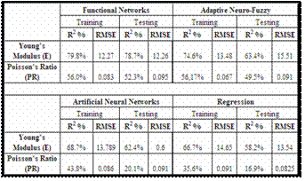
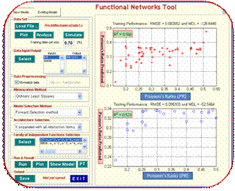
Figure 5: Data with 77 samples: Poisson’s Ratio versus its predicted values based on Functional networks with polynomial basis of degree at most 3.

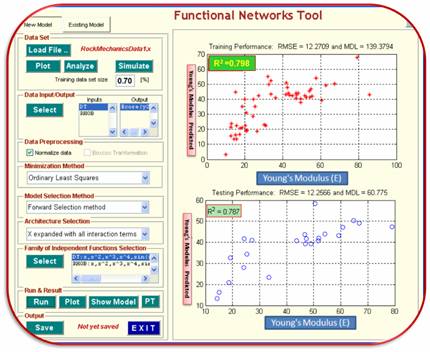
Figure 6: Data with 77 samples: Young’s Modulus versus its predicted values based on Functional networks with polynomial basis of degree at most 3.

Figure 7: Data with 51 samples: Unconfined Compression Strength (UCS) versus its predicted values based on Functional networks with polynomial basis of degree at most 3.

Conclusion
In this research, we have investigated functional networks capabilities in predicting rock mechanical parameters for hydrocarbonate reservoirs. Functional networks outperform the most common existing predictive models, especially, multilayer perceptron feedforward neural networks, statistical regression, and adaptive neuro-fuzzy inference sytems. Functional networks have the the highest R2 and smallest root mean squared erros in the case of predicting both Young’s Modulus and Poisson’s  ratio with adequate computational time.
The work can be extended to include: (i) more experimental data with uncertain numerical attribute measurements; (ii) different set of linearly independent families and genetic algorithms.  This will make the framework more robust and reliable.

Acknowledgement
The authors would like to acknowledge the support provided by King Abdulaziz City for Science and Technology (KACST) through the Science & Technology Unit at King Fahd University of Petroleum & Minerals (KFUPM) for funding this work under Project No. 08-OIL82-4 as part of the National Science, Technology and Innovation Plan. We wish to thank MEDai Inc., an Elsevier Company for their support and facilities required for this research.

References

1. Abdulraheem A., Ahmed M., Vantala A., Parvez T., “Prediction of Rock Mechanical Parameters for Hydrocarbon Reservoirs Using Different Artificial Intelligence Techniques”. The 2009 SPE Saudi Arabia Section Technical Symposium and Exhibition, Alkhobar, Saudi Arabia, 9-11 May 2009. SPE 126094.
2. Abdulraheem A., El-Sebakhy E., Ahmed M., Vantala A., Raharja I., and G.  Korvin, “Estimation of Permeability from Wireline Logs in a Middle Eastern Carbonate Reservoir Using Fuzzy Logic”.  The 15th SPE Middle East Oil & Gas Show and Conference held in Bahrain International Exhibition Centre, Kingdom of Bahrain, 11–14 March 2007.  SPE 105350. 
3. El-Sebakhy E. A., Abdulraheem A., Ahmed M., Al-Majed A., Raharja P., Azzedin F., and Sheltami T., “Functional Networks as a Novel Approach for Prediction of Permeability and Porosity in a Carbonate Reservoir”, the 10th Int. Conference on Eng. Applications of NNs  EANN2007,  Thessaloniki, Hellas, Greece. (29-31 August, page(s) 422-433, 2007. 
4. Osman E., Al-Marhoun M., “Artificial Neural Networks Models for Predicting PVT Properties of Oil Field Brines", paper SPE 93765, 14th SPE Middle East Oil & Gas Show and Conference in Bahrain, March 2005.
5. Castello E., Functional networks. Neural Proc. Lett. 7 (1998), pp. 151-159.
6. El-Sebakhy E. A., Hadi S. A., and Faisal A. K.., (2007), “Iterative Least Squares Functional Networks Classifier”. IEEE Transactions Neural Networks, vol.3, May 2007, 844-850.
7. El-Sebakhy E. A., (2008), “Software Reliability Identification Using Functional Networks: A Comparative Study”. International Journal of Expert Systems with Application. August 2008, 411-424.
8. El-Sebakhy E., Faisal K., El-Bassuny T., Azzedin F., and Al-Suhaim A., (2006), “Evaluation of Breast Cancer Tumor Classification with Unconstrained Functional Networks Classifier”; the 4th ACS/IEEE International Conf. on Computer Systems and Applications. 281-287.
9. Siggins, A.F. (1993). Dynamic Elastic Tests for Rock Engineering. Comprehensive Rock Engineering (Eds: J.A. Hudson, E.T. Brown, C. Fairhurst, and E. Hoek). Pergamon Press. UK.
10. Hilbert, L.B., T.K. Kwong, N.G.W. Cook, KT Nihei and L.R. Myer. (1994). Effects of strain amplitude on the static and dynamic non-linear deformation of Berea sandstone. Proceedings of the 1st North American Rock Mechanics Symposium, pp. 497-502.
11. Plona T.J. and J.M. Cook (1995). Effects of stress cycles on static and dynamic Young's moduli in Castlegate sandstone. Rock Mechanics. Daamen & Schultz (editors). Balkema. Rotterdam.
12. Suarez-Rivera, R.S. Nakagawa, L. and R. Myer (1997). Determination of Rock Elastic Properties from Acoustic Measurements of Rock Fragments. Int. J. Rock Mech. & Min. Sci. Vol. 34; No.3-4. Paper No.304.
13. Ahmed, U., M.E. Markley, and S.F. Crary (1991). Enhanced In Situ Stress Profiling with Microfracture, Core and Sonic Logging Data. SPE 19004, SPE Formation Evaluation, June 1991, pp. 243-251.
14. Gattens III, J.M., C.W. III Harrison, D.E. Lancaster, and F.K. Guidry (1990). In-Situ Stress Tests and Acoustic Logs Determine Mechanical Properties and Stress Profiles in the Devonian Shales. SPE Formation Evaluation, Sept. 1990, pp. 248-254.
15. Raaen, A.M., K.A. Hovem, H. Joranson, and E. Fjaer (1996). FORMEL: A step forward in strength logging. SPE paper no 36533 presented at the 1996 SPE Annual Technical Conference and Exhibition, Denver, CO.
16. Murillo, A., J. Neuman, and R. Samuel (2001). Estimation of Rock Dynamic Elastic Property Profiles through a Combination of Soft Computing, Acoustic Velocity Modeling, and Laboratory Dynamic Test on Core Samples. SPE Asia Pacific Oil and Gas Conference and Exhibition, 17-19 April 2001, Jakarta, Indonesia.
17. Nikravesh, M. (1998). Neural Network Knowledge-Based Modeling of Rock Properties Based on Well Log Databases. SPE Western Regional Meeting, 10-13 May 1998, Bakersfield, California.
18. Badarinadh,, V., Suryanarayana, K., Youssef, F.Z., Sahouh, K., Valle, A., 2002. Log-Derived Permeability in a Heterogeneous Carbonate Reservoir of Middle East, Abu Dhabi, Using Artificial Neural Network. SPE 74345, International Petroleum Conference and Exhibition in Mexico, Villahermosa, Mexico.
19. Simon, H., 1994. Neural Networks- a Comprehensive Foundation. Macmillan Publishing Englewood Cliffs, NJ, USA.
20. Hambalek, N., Reinaldo, G., 2003. Fuzzy logic applied to lithofacies and permeability forecasting. In: Proceedings the Society of Petroleum Engineering (SPE). Latin America and Caribbean Petroleum Engineering Conference, Spain, Trinidad, West Indies, SPE paper 81078.
21. Cuddy, S., (1998). Litho-facies and permeability prediction from electrical logs using fuzzy logic.  In: Proceedings the Society of Petroleum Engineering (SPE), Abu-Dhabi International Petroleum Exhibition and Conference, (ADIPEC), Abu Dhabi, UAE, SPE paper 49470.

AAPG Search and Discovery Article #90105 © 2010 AAPG GEO Middle East Conference & Exhibition, Manama, Bahrain, 7-10 March 2010